Consumer Demand and Labor Supply in
Sweden
Bengt Assarsson
Department of Economics
Uppsala University
Box 513,
Sweden
Abstract
This paper analyses the demand for consumer goods and leisure in Sweden for the period
1Introduction
The estimation of demand elasticities has a long tradition in applied economics. During the 1970ies and 1980ies demand systems based on speci…c utility or cost functions were estimated and e¤ort was put on deriving attractive functional forms of these systems. The most successful demand systems were those with a ‡exible functional form, such as the Translog1 or the AIDS (Almost Ideal Demand System)2 . Demand systems were often estimated with aggregate time series data, though the theory from which the systems were derived considered the behavior of a single consumer or household. Initially, systems like the Translog and AIDS were static. Later, dynamic versions of these models were used and …t the data better.
The purpose of this paper is to estimate demand elasticities for the most recent Swedish aggregate consumption data. The elasticities can be used for example for estimating deadweight losses for di¤erent tax schedules or for computing optimal tax rates according to the Ramsey or inverse rule3 , i.e. tax rates being set inversely to the compensated price elasticity of demand4 . These elasticities must also include the price elasticities (own and cross price elasticities) of leisure time. If leisure time is excluded, the implicit assumption is that the
The paper is organized as follows. The next section gives a brief introduction to the theory of consumer demand and some of the problems that occur in this type of exercise. The third section discusses the problems of specifying the demand system, which in this case is a dynamic version of the AIDS model. The fourth section gives a detailed description of the data and how the treatment of leisure time is done. The …fth section gives the main empirical results, while detailed tables can be found in the Data appendix. The last section gives the conclusions.
2Theory of consumer demand
A general description of the consumer’ decision problem is given in the life cycle hypothesis. There, the consumer maximizes expected discounted utility from a bundle of consumption goods and services as well as leisure time - given an intertemporal budget constraint. With many goods and services and demand dependent on many expected future discounted prices this problem becomes very complex and di¢ cult to handle in empirical applications. Various assumptions have to be done in order to keep the problem manageable. Rather than starting from the most general and compley theory, here the most simple static model is used but extended with some dynamics. This is one of the ways in which the
1 See Christensen, Jorgensen and Lau (1979).
2 See Deaton and Muellbauer (1980).
3 See Atkinson and Stiglitz (1980), p. 369.
4 The compensated price elasticity of demand for good i with respect to a change in the
| pj | ||||||||||
| @ q i | ||||||||||
| price of good j is de…ned as "ij = | , where qi | belongs to a bundle of goods, | q | , which | ||||||
| @pj | q | i | ||||||||
| gives the same utility as before the price change, i.e. | 0 | ): | ||||||||
| u(q ) = u(q | ||||||||||
1
development has proceeded in the literature5 .
Generally, the consumer maximises the expected utility
| T t | |
| X | |
| max (1 + r) (1+ )Et fu(qt+ )g | (1) |
| =0 | |
| subject to an intertemporal budget constraint | |
| At+1 = At + !tht ptqt | (2) |
where the horizon is from t to T, r is the real rate of interest, is the rate of time preference, E is the expectations operator, u is the utitilty function, At is wealth at time t, !t is the wage rate, ht is the number of hours worked, pt = p1t; :::; pnt is a vector of prices and qt = q1t; :::; qnt a vector of quantities. Assuming intertemporal separability, and for convenience dropping the time subscript, the problem can be stated
X
| max u(q) subject to x = | piqi | (3) |
where x is total expenditure. The solution to this problem gives the Marshallian demand functions qi = gi(x; p). If these demand functions are substituted into the direct utility function u(q) the indirect utility function u = '(x; p) is obtained. The indirect utility function shows the highest possible utility that can be attained for alternative prices and total expenditure. The dual problem is to minimize the total expenditure required to obtain a given utility level, which can be stated as
| min x = pq | (4) |
| subject to | |
| u = v(q) | (5) |
The solution to this problem gives the Hicksian demand functions as qi = hi(u; p) which may simply be derived as the partial derivative of the cost function x = c(u; p) w.r.t. pi. The cost function shows the minimum cost to obtain utility level u at prices p. Substituting the indirect utility function (which is the inverse of the cost function) into the Hicksian demand functions gives the Marshallian demand functions. In this paper the dual approach to obtain the demand functions is used.
The total expenditure elasticity is de…ned as Ei = @qi x and shows the percentage change of the demand for good i following a one percentage change in total expenditure (often also referred to as the income elasticity). Letting
wi = denote the budget share of the
P
property that wiEi = 1: The uncompensated6 price elasticity of demand is
de…ned as eij = @qi pj and shows the percentage change of the demand for good i
@pj qi
following a one percentage change in the price of good j. For i = j we refer to the
5 See Deaton and Muellbauer (1980b) and Edgerton et al (1996) where various dynamic versions of the AIDS model were developed.
6 Uncompensated implies that the consumer is not compensated for the loss in income induced by a price increase.
2
P
property is that j eij + Ei = 0: Finally, the compensated7 price elasticity is
s
de…ned as eij = eij + wj Ei which shows the percentage change of the demand for good i following a one percentage change in the price of good j - at constant utility.
2.1Static and dynamic model
The consumer’ decision problem with respect to both consumption goods and leisure is dynamic and is probably best analysed within the
consumption items, i.e. the demand functions could be stated in terms of marginal utility as qi = hi ( @u@c ; p) , as in Blundell et al (1994). However, here we
follow the simpler route and introduce simple dynamics in an otherwise static framework.
Particular problems also arise in the context of durable goods, i.e. goods which are not consumed within the data period one quarter of a year. The consumption of Housing is for rental apartments estimated as rents in nominal and …xed prices, while for
2.2Utility tree and
The number of goods available to the consumer and the number of observations present in the data obviously poses a problem, particularly to the researcher occupied with
7 Compensated implies that the demand is calculated at the point where the consumer is compensated for the loss in income induced by the price change so that the utility is the same as before the price change. The compensated demand hence measures the pure price e¤ect.
8 See Gorman (1959), Pollak (1971), Deaton and Muellbauer (1980a, Ch. 5.2), Pudney (1981), Varian (1982), Laisney (1991) or Edgerton et al.(1996).
3
are said to be weakly separable if they can be represented by a utility function of the form
| u = f [v1(q1); :::; vn(qn)] | (6) |
where qr represents the vector of quantities in the rth group. Utility maximization now means maximizing the functions vr(qr) separately, using the standard tools of demand analysis but replacing total expenditure by group expenditure xr: The Marshallian demand functions now can be written
| qri = gri(p1; :::; pn; xr) | (7) |
P
where pr denotes the price vector of the rth group and xr = i priqri is the total expenditure of the group. The …rst stage allocation of total expenditure into group expenditure is a problem since the price vectors pr must be replaced by some price indices pr: Deaton and Muellbauer (1980a) show that an approximation exists such that the demand function above can be replaced by
| Qr = gr(P1; :::; Pn; x) | (8) |
where Qr is a quantity index - or expenditures expressed in constant prices - and Pr a price index, where the latter could be an approximation to a true cost of living index. Though the assumption of weak separability means that one can study the consumer’ optimization problem at separate stages it has implications for the e¤ect of a price change on a certain group belonging to group r on the demand for another good belonging to another group s. In addition, the expenditure elasticity depends both on the …rst stage elasticity and the elasticity within the group at lower stages of the budgeting process. If a price of a particual good increases it will a¤ect the demand for all goods in the group to which the good belong. But the price index of the group - Pr - is also a¤ected and hence the demand for all other goods belonging to groups outside r. The relationships are uncovered in Edgerton (1992, 1993) and Edgerton et al (1996, p.
| Pr = | c(u; pr) | ||
| c(u; ) | |||
| where is the unit vector, xr = PrQr, x = | r xr | ||
| substitution we obtain the Marshallian demand | as | ||
| P | |||
(9)
P
and Qr = i Qri. By
| qri = gri [pr; Prgr(P1; :::; Pn; x)] = gri(p1; :::; pn; x): | (10) |
Following Edgerton et al (1996) and using the de…nitions E(r)i for the within group expenditure elasticity, E(r) for the group expenditure elasticity, and Ei for the total expenditure elasticity and similarly for price elasticities - eij for the
uncompensated and eij for the compensated price elasticity - and budget shares we obtain the following de…nition of elasticities:
| Ei | = E(r)E(r)i | (11) |
| eij | = rse(r)ij + E(r)iw(s)j ( rs + e(r)(s)) | |
| = rs eij + E(r)iw(s)j e(r)(s) | ||
| eij | = rs e(r)ij | + E(r)iw(s)j e(r)(s) |
4
where rs = 1 for r=s and zero otherwise9 . How should these de…nitions be interpreted? The expenditure elasticities are straightforward. The price elasticity is composed of two parts which can be labelled the direct and indirect e¤ects. The direct e¤ect - rse(r)ij - is the within group price elasticity measured in the usual way. The indirect e¤ect measures how much the price change of a certain good a¤ects the allocation among groups. It depends on the three factors
E(r)i - the within group expenditure elasticity
w(s)j - the budget share of the good which price changes andrs + e(r)(s) - the price elasticity between groups r and s
The …rst factor measures the e¤ect of the change in group expenditure (due to the price change) on the expenditure on the ith good. The second factor measures the relative change of the group price index caused by the change of the price of the ith good, which is measured by the budget share of the price changing good. The third factor measures the e¤ect on the demand for group r - on Qr - of a change in the price index of group s - of Pr.
Note that if the latter own price elasticity equals
proportional change in the expenditure of the group and eij = e(r)ij : Note also that the total price elasticity is well approximated by the within group price elasticity if the within group budget share of the price changing good is small or within group expenditure elasticities are small.
3Speci…cation of demand system
The estimation of elasticities requires a speci…cation of the demand model. Several alternatives exist in the literature. In Edgerton et al (1996) di¤erent speci…- cations are evaluated empirically. The …nally chosen model is the AIDS (Almost Ideal Demand System) model which is commonly applied in the empirical literature.
3.1 The AIDS model
| The AIDS uses the time period t cost function | Y | |||||
| X | 1 | XX | ||||
| log c(ut; pt) = 0 + k log pkt + | log pkt log pjt +u | 0 | p k | (12) | ||
| 2 | kj | kt | ||||
| k | k j | k | ||||
where u is the utility level, p is a price vector, pkt is the price of the
As described in section 2, taking the partial derivative w.r.t. the
9 rs is the so called Kronecker’s delta.
5
| wit = i + Xj | ij log pjt + i (log xt log Pt ) | ||||||||||||||
| where P | = 0 | + | k | k log pkt+ 1 | k j | kj | log pk log pj : | kj | = 1 | ||||||
| t | 2 | 2 | ij | ||||||||||||
| and wit = | pitqit | the budget share for the |
|||||||||||||
| pjtqjt | |||||||||||||||
| P | |||||||||||||||
(13)
+ ji
3.2Linear AIDS
A linear version of the AIDS model was suggested by Deaton and Muellbauer (1980) where the price index Pt was replaced by the index
X
| Pt = 0 + wkt log pkt | (14) |
| k |
This approximation has become very popular in the literature. Here, both linear and nonlinear versions have been used. Though the linear version of AIDS has proven accurate in a number of studies10 I have …nally chosen the nonlinear version. The additional computational burden is small and the results not particularly sensitive to the a priori choice of the parameter 0.11 . The linear version was evaluated here but it was the nonlinear version that was …nally chosen.
3.3Dynamic AIDS
The simplest static model is not likely to perform well with time series data. Di¤erent dynamic versions of the model have been used in the literature. A
dynamic demand system suggested by Assarsson (1991), Alessie and Kapteyn (1991) and Kesavan et al (1993) can be derived from a dynamic form of the cost function. Using the principle of demographic translation, as suggested by Pollak and Wales (1981), results in demand functions
XX
wit = i + ij wjt 1 + ij log pjt + i (log xt log Pt ) (15)
jj
where
| 0 | X | 1 | X | XX | (16) | |||||||||||||||||||||||
| P | X@ | A | 1 | |||||||||||||||||||||||||
| = | 0 | + | k | + | kj | w | jt 1 | + | k | log p | kt | + | kj | log p | k | log p | j | |||||||||||
| t | k | j | k | 2 | k j | |||||||||||||||||||||||
| This type of system was evaluated here and short and long run elasticities | ||||||||||||||||||||||||||||
| were derived. The restriction | k kj | = | j kj | = 0 was used, where the …rst | ||||||||||||||||||||||||
| 10 | Alston et al (1994),Buse (1994) or Edgerton et al (1996). | |||||||||||||||||||||||||||
| See for example Chalfant (1987),P | P | |||||||||||||||||||||||||||
11 The parameter 0 was set to 30 percent of the log of total expenditure in 1995, the base year in which prices was normalised to unity.
6
sum implies
3.4AIDS in error correction form
Another alternative, which was …nally chosen, is the error correction form, which has become very popular recently and seems to …t the data well. It allows both short term and long term as well as feedback responses to be estimated and it can be derived from the basically static AIDS framework through the method of demographic translation. The long run equilibrium can be desribed by (13) above and the error correction form as
| w | = | Xj {ij log pjt + 'i | log(x=P ) + | (17) | |||||||||
| it | 1 | t | Xj | ij it 1 | |||||||||
| where Pt | X | XX | (18) | ||||||||||
| = | 0 + k log pkt + | kj log pk log pj | |||||||||||
| k | 2 | k | j | ||||||||||
| kj | = | 1 | ij + ji | (19) | |||||||||
| 2 | |||||||||||||
| and it 1 | = | wit 1 i Xj | ij log pjt 1 i (log xt 1 log Pt 1)(20) | ||||||||||
The matrix should be restricted in order for the system to be theoretically
| consistent. In particular, it is su¢ cient if i ij = | j ij = 0 for adding up and |
| be coherent (and possible to estimate | |
| identi…cation to hold. For the system to P | P |
e.g. with Full Information Maximum Likelihood) parameters have to be further restricted. Di¤erent speci…cations were tested and the …nally chosen system is a restricted version which allows six commodity groups to be included. The preferred speci…cation use a single scalar as the error correction term. The model can be rewritten in level form as
| wit = i + Xj {ij log pjt + 'i log(x=P )t + (1 + )wit 1 + | |
| Xj ij log pjt 1 + i log(x=P )t 1 | (21) |
which can be derived from the AIDS expenditure function (12) by translating the parameter i into
| i = i + (1 + )wit 1 + Xj kj log pjt 1 + i log(x=P )t 1 | (22) | ||||||||
| and the long run parameters be derived as | |||||||||
| ij | = | {ij + ij | ; | i | = | 'i + i | : | (23) | |
This is the speci…cation …nally used for estimating the elasticities and can be viewed as a compromise which on the one hand saves parameters through
7
various restrictions derived from economic theory but on the other hand is ‡exible enough to allow for the most important dynamics.
3.5Elasticities
The long run elasticities in the model are then given by (22) - (26):
| l | i | |||||||||||
| Ei | = | 1 + | ||||||||||
| wi | ||||||||||||
| l | ij | i | j + | 21 | k kj + jk | log pk | ||||||
| eij | = | Pwi | ij | |||||||||
| elij | = eijl + wj Eil | |||||||||||
and the short run elasticities by (27) - (29):
| s | 'i | ||||||||||
| Ei | = | 1 + | |||||||||
| wi | |||||||||||
| s | {ij | 'i | j + 1 | k ({kj + {jk) log pk | |||||||
| eij | = | 2 | Pwi | ij | |||||||
| s | = | s | s | ||||||||
| eij | eij | + wj Ei | |||||||||
(24)
(25)
(26)
(27)
(28)
(29)
where ij is Kroneckers delta. Seasonal dummies are included in the estimations but for simplicity have been excluded in the formulas above.
Note that the short run elasticities are not directly identi…ed due to the loss of the constant term in the di¤erence form. The parameter i is interpreted as the budget share for a household at the subsistence level and is identi…ed in the derivation of the long run elasticities. The short run elasticities are identi…ed by assuming that i in the short run is equal to the long run value.
4Data
The data used is quarterly national accounts running from
12 Compensated
8
4.1Utility tree and speci…cation of categories
With quarterly data for the period
The design of the
Table 1. Goods in
| 1 | Food, beverages, and health care | 1_1 | Food including light beer |
| 1_2 Alchohol and tobacco | |||
| 1_3 | Restaurant | ||
| 1_4 | Health care | ||
| 2 | Housing, fuel, and furniture | 2_1 | Housing, fuel, and furniture |
| 3 | Household and personal care | 3_1 | Clothing and shoes |
| 3_2 | Household utensils | ||
| 3_3 Post and telephone | |||
| 3_4 | Hotels | ||
| 4 | Transports, vacation travel | 4_1 | Vehicles including fuel |
| 4_2 | Transports | ||
| 4_3 Foreign travel and consumption | |||
| 4_4 Recreation including cultural activities | |||
| 5 | Miscellaneous goods and services | 5_1 | Goods for recreation |
| 5_2 | Games | ||
| 5_3 Books and magazines | |||
| 5_4 | Miscellaneous goods | ||
| 5_5 | Insurance | ||
| 6 | Leisure | 6_1 | Leisure |
with budgeting in two stages. The
4.2The measurement and treatment of leisure
Suppose the
budget share of leisure then is wn = Ppnqn : The price of leisure has been
j pj qj
9
measured as the wage rate less the average marginal tax rate13 . The budget restriction then can be written
Xn 1
| piqi = pnh + A; | (30) |
| i=1 |
where pnh is labor income, h is the total number of hours worked and A is
Xn
| i=1 piqi = pn(T ml z s n) + A M | (31) |
where M usually is referred to as full or potential income15 . The problem then is how to estimate leisure time. The daily budget for an individual consumer could simply be determined as
The number of daily hours is then aggregated to the total number of quarterly leisure hours for the adult population, b. The conversion factor from daily to quarterly hours is , the number of days each quarter. These have been estimated as the number of ordinary working days, i.e. …ve days for an ordinary week and also exclusive of all "red" days. The simplest measure of the total number of quarterly leisure hours is therefore (24 8) b ml. However, we also assume that some of the time of the unemployed is used for home production and labor search. If the the number of unemployed persons are labelled u, then the labor force is l + u and we assume that 1mu hours is used for home production and labor search. Similarly, we assume that the elderly - or the adult population outside the labor force - use some time for home production and labor search, which is 2m(b (l + u)). Finally, there is the number of subsistence hours, which are related to sleeping, eating and for some health care, etc. which are di¢ cult to determine. We denote this by bn. The total number of quarterly leisure hours then can be determined as
| 24 b ml 1mu 2m(b (l + u)) nb | (32) |
where the respective terms are
13 The hourly compensation paid by employers have been obtained as the total compensation divided by the total number of hours worked, as described in the National Accounts. The data on average marginal tax rates have been obtained from Gunnar du Rietz, Ratio. The relative
| wage | (1 t2) | 1 t2 | 1 t2 | |||||
| price of leisure is determined by | (1+t1) | = wage | = pn where | |||||
| pf (1+t3) | ||||||||
| pf | (1+t1)(1+t3) | pi | (1+t1)(1+t3) | |||||
is the total tax wedge., where wage is the compensation paid by the employer, t1 is the payroll tax rate, t2 is the income tax rate and t3 is the indirect tax rate. All prices in this study are measured including indirect taxes and wages excluding payroll taxes. The price on leisure is therefore simply the wage rate net of the average marginal tax rate.
| 14 | The simplest formulation would be to use the budget restriction | P | n | ||
| i=1 piqi = pnT + A; | |||||
| for T = h + q | n | : | |||
| 15 | |||||
| See Dowd (1992) or Madden (1995) for similar treatments. | |||||
16 An alternative would be to measure
T = 24.
10
24 b= the total number of hours available ml= the number of hours worked
1mu= the number of hours worked in home production and labor search by those unemployed
2m(b (l+u))= the number of hours worked in home production and labor search by those outside the labor force
nb= the number of subsistence hours worked in home production, sleeping, etc. by the adult population
The formula can be simpli…ed to
| (24 n) b m [l 1u 2(b (l + u))] | (33) |
Data are available on all variables less i and n, for which some assumptions are necessary. The basic assumption is ( 1 = 0:5; 2 = 0:2; n = 12). For a fully employed person this means that the daily leisure time is
5Empirical results
5.1Estimated equations
The empirical results are presented extensively in the data appendix. Here some summary results from the estimations are presented. In general the goodness of …t of the estimated equations are satisfactory, which can be seen in Table 2.
11
Table 2. Summary statistics for estimated demand systems.
| 2 | Mean of | Standard error | |||
| System | dep. var. | of regression | autocorrelation test | ||
| R | |||||
| Stage 1: 1 | 0.97 | 0.15 | 0.0036 | 0.08 | |
| 2 | 0.95 | 0.16 | 0.0037 | 0.31 | |
| 3 | 0.95 | 0.08 | 0.0029 | 0.08 | |
| 4 | 0.70 | 0.11 | 0.0060 | 0.08 | |
| 5 | 0.94 | 0.07 | 0.0031 | 0.63 | |
| 6 | 0.97 | 0.43 | 0.0065 | 0.68 | |
| Group 1: 1_1 | 0.90 | 0.65 | 0.0077 | 0.01 | |
| 1_2 | 0.79 | 0.18 | 0.0059 | 0.36 | |
| 1_3 | 0.78 | 0.14 | 0.0088 | 0.02 | |
| 1_4 | 0.96 | 0.03 | 0.0016 | 0.18 | |
| Group 2: 2_1 | 0.95 | 0.16 | 0.0037 | 0.31 | |
| Group 3: 3_1 | 0.55 | 0.47 | 0.0130 | 0.11 | |
| 3_2 | 0.41 | 0.40 | 0.0093 | 0.11 | |
| 3_3 | 0.79 | 0.11 | 0.0057 | 0.29 | |
| 3_4 | 0.91 | 0.03 | 0.0010 | 0.14 | |
| Group 4: 4_1 | 0.89 | 0.56 | 0.0127 | 0.82 | |
| 4_2 | 0.68 | 0.11 | 0.0043 | 0.05 | |
| 4_3 | 0.85 | 0.23 | 0.0130 | 0.19 | |
| 4_4 | 0.96 | 0.10 | 0.0031 | 0.13 | |
| Group 5: 5_1 | 0.92 | 0.42 | 0.0098 | 0.03 | |
| 5_2 | 0.89 | 0.11 | 0.0064 | 0.11 | |
| 5_3 | 0.98 | 0.14 | 0.0050 | 0.07 | |
| 5_4 | 0.72 | 0.25 | 0.0067 | 0.00 | |
| 5_5 | 0.92 | 0.08 | 0.0034 | 0.04 | |
| Group 6: 6_1 | 0.97 | 0.43 | 0.0065 | 0.68 | |
The …rst column shows the goodness of …t of the individual equations in
2
each system. In stage 1 R for all equations except Transports are around 0.95. For Transports it is 0.70. The second column shows the mean of the dependent variable revaling that the mean of the budget share of goods consumption for
Turning to Stage 2 it can be noted that the …t is generally somewhat lower. In Group 1 Food is the biggest category, accounting for 65 percent within the
group and totally (0.65 0.15) 100 = 9.8 percent with a 0.8 percent standard
2
error. The R = 0:9 for Food but there is some autocorrelation in this equation.
17 See Engle (1984).
12
However, the other equations in Group 1 show no sign of autocorrelation so that autocorrelation in the group as a whole can be statistically rejected.
The …t of the Housing - Group 2 - equation is 0.95 and the standard error is 0.4 percent. The budget share is 16 percent, 28 percent of total consumption (less leisure). In Group 3 autocorrelation is rejected in all equations. However, the …t is rather poor in this group. In Group 4 there is autocorrelation in 4_2 - Transports. The …t is rather poor in this category - 0.68. Finally, in Group 5 there is autocorrelation in three of the …ve groups: 5_1, 5_4 and 5_5, while there is no sign of autocorrelation in the aggregate as revealed in the equation for Group 5 in the Stage 1 estimation.
5.2Estimated elasticities
Estimated elasticities are presented in the data appendix. Here, some summary results are presented. In Table 3, the total elasticities de…ned in (11) are shown. The
Table 3. Total long run compensated
| Compensated | Total expen- | |
| diture | ||
| Item | elasticity | elasticity |
| Food including light beer | 0.55 | |
| Alchohol and tobacco | 0.58 | |
| Restaurant | 0.96 | |
| Health care | 0.53 | |
| Housing, fuel, and furniture | 0.21 | |
| Clothing and shoes | 2.61 | |
| Household utensils | 2.65 | |
| Post and telephone | 1.80 | |
| Hotels | 2.29 | |
| Vehicles including fuel | 2.30 | |
| Transports | 2.99 | |
| Foreign travel and consumption | 5.40 | |
| Recreation including cultural activities | 2.93 | |
| Goods for recreation | 2.35 | |
| Games | 1.83 | |
| Books and magazines | 1.94 | |
| Miscellaneous goods | 1.69 | |
| Insurance | 4.62 | |
| Leisure | 0.49 |
All compensated
13
Books and magazines. The VAT on books were recently reduced from 25 to 6 percent which eventually would lower prices by some 15 percent and consequently increase demand by almost 25 percent in the long run (the compensated
Table 4. Total short run compensated
| Compensated | Total expen- | |
| diture | ||
| Item | elasticity | elasticity |
| Food including light beer | 0.30 | |
| Alchohol and tobacco | 0.59 | |
| Restaurant | 0.82 | |
| Health care | 0.38 | |
| Housing, fuel, and furniture | 0.23 | |
| Clothing and shoes | 1.50 | |
| Household utensils | 1.37 | |
| Post and telephone | 1.27 | |
| Hotels | 1.22 | |
| Vehicles including fuel | 2.16 | |
| Transports | 0.80 | |
| Foreign travel and consumption | 0.84 | |
| Recreation including cultural activities | 1.00 | |
| Goods for recreation | 1.18 | |
| Games | 0.92 | |
| Books and magazines | 0.98 | |
| Miscellaneous goods | 0.85 | |
| Insurance | 2.32 | |
| Leisure | 1.23 | |
Table 4 shows the corresponding short run elasticities. These are the direct e¤ects of changes in prices and total expenditure, i.e. that occur within a quarter. In most cases the absolute value of the elasticity is smaller in the short than in the long run. This supports the interpretation of adjustment costs or habit formation in the demand for these goods. This applies to all total expenditure elasticities except Leisure for which the short run elasticity is 1.23 - a luxury - while being only 0.49 in the long run - a necessity. The short run compensated
Why would the short run elasticity overshoot and exceed the long run elasticity? This would likely occur for goods where demand is very ‡exible and the degree of habit formation low. These e¤ects are particularly strong for Clothing and shoes, Household utensils, and Hotels. For these categories the response to a change in the relative price has a large immediate e¤ect but declines in the long run. For the categories Housing, Transports and Miscellaneous the initial response is instead relatively small but increases to reach a peak at the long run value.
14
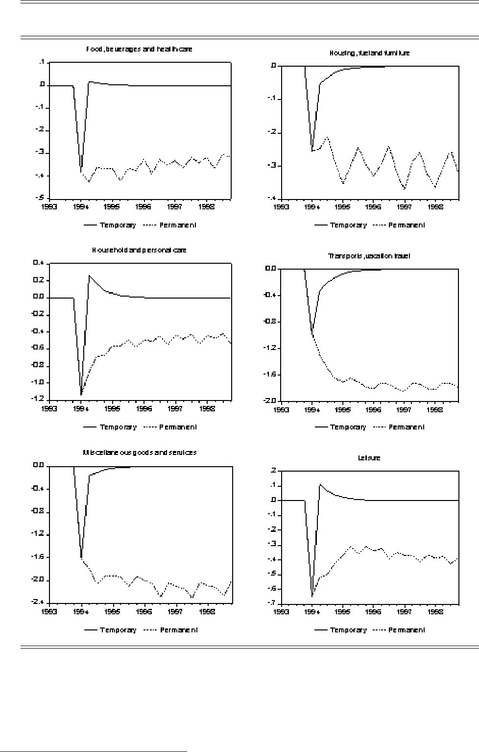
Figure 1. Short and long run
We can distinguish not only between long and short run elasticities but also between the response to temporary and permanent changes in prices and total expenditure (full income). In Figure 1 the dynamic response to relative price changes are shown. The charts show the
18 The shocks are
15
in Stage 1 and given in Table B1 in the data appendix. A temporary price change has a temporary demand e¤ect which lasts for about 2 years. The overshooting property can be seen particularly for Household and personal care and Leisure. The response which could be expected due to the presence of adjustment costs can be noticed in particular for Housing, fuel and furniture, Transports and vacation travel and Miscellaneous goods and services.
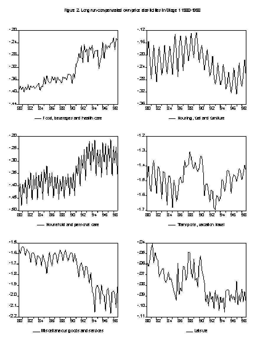
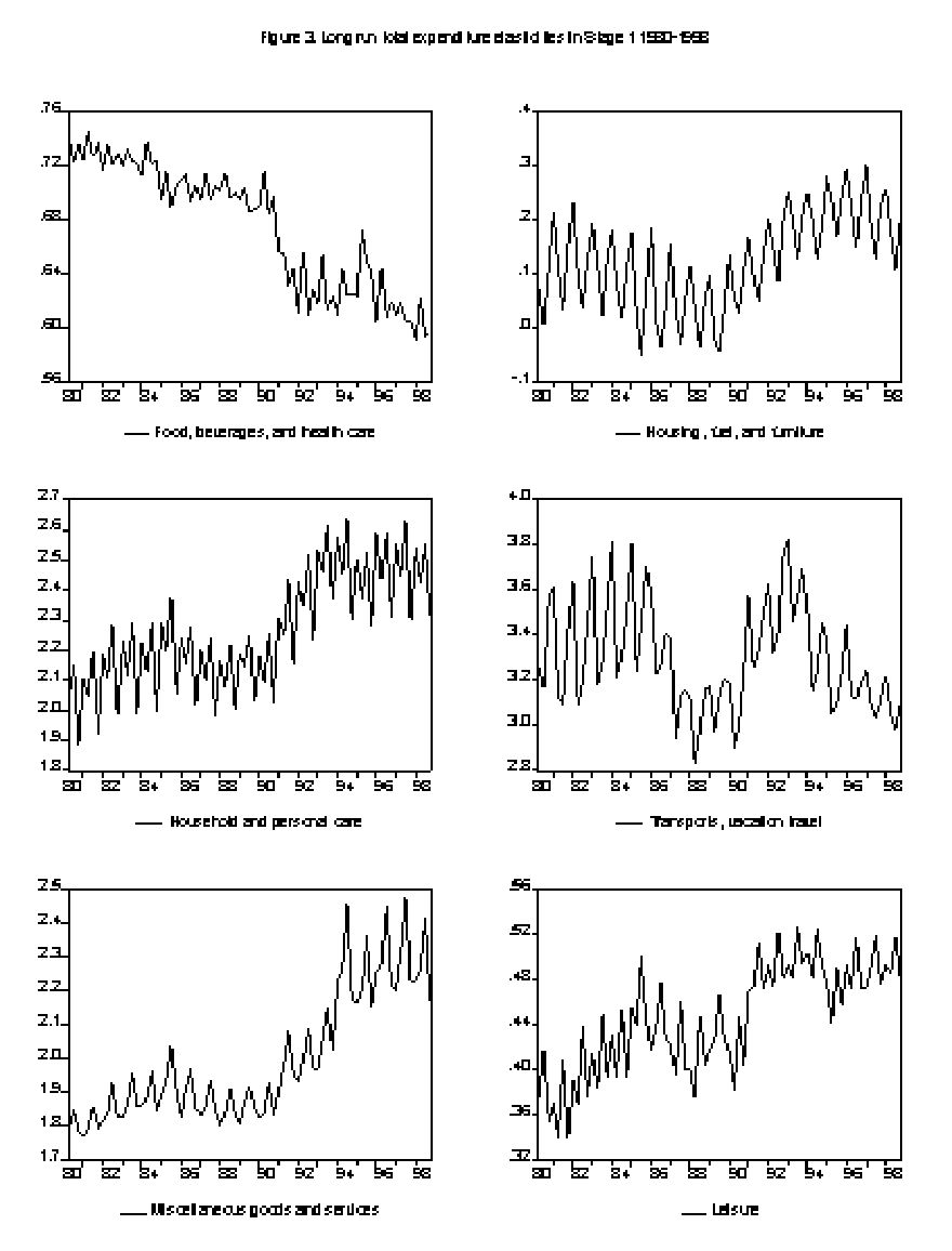
The elasticities also vary over time due to variations in budget shares, prices and full income, as apparent from the de…nitions of elasticities in (22) - (29). These variations are illustrated in Figures 2 and 3 which show long run compensated
As can be seen in Figure 2 the long run compensated
In Figure 3 the long run total expenditure elasticities are shown. They are all positive and lowest for the Food, Housing and Leisure categories. The elasticity drops from about 0.75 to 0.6 for Food, increases from .1 to .2 for Housing and from .4 to .5 for Leisure. Though the elasticities vary they are fairly stable during the sample period.
5.3Labor supply elasticities
The responses shown in Figure 1 indicate that the initial labor supply response is quite large but declines in the long run. The short run uncompensated response is about
It is interesting to compare the results for demand systems with and without Leisure, since the measurement of Leisure in itself seems uncertain. We do that by estimating the Stage 1 demand system with and without Leisure. The results are presented in Table 5.
19 Surveys of labor supply are Pencavel (1986) and Killingsworth and Heckman (1986).
16
17
18
Table 5. Comparison of uncompensated price
and total expenditure elasticities with and without Leisure in Stage 1. At mean values
| 1 | 2 | 3 | 4 | 5 | 6 | |
| 1 | 0.53 | |||||
| 0.09 | 0.19 | 0.17 | ||||
| 2 | 0.07 | 0.05 | 0.33 | |||
| 0.08 | 0.11 | |||||
| 3 | 0.53 | 0.15 | ||||
| 0.25 | 0.21 | 0.47 | ||||
| 4 | 0.31 | 0.11 | ||||
| 0.34 | 0.13 | 0.15 | ||||
| 5 | 1.09 | 0.04 | 0.18 | 0.23 | ||
| 0.82 | 0.25 | |||||
| 6 | 0.11 | |||||
| x/P | 0.62 | 0.21 | 2.47 | 3.19 | 2.27 | 0.49 |
| 0.45 | 0.53 | 1.45 | 1.80 | 1.50 | ||
First, the classi…cation of necessities and luxuries are the same20 , though the total expenditure elasticities are higher particularly for the groups 3, 4, and 5. This depends on Leisure being classi…ed as a necessity with a large budget share.
5.4Comparison with previous results
The results are compared to previous empirical results in Table 6. The table is incomplete and only presents a small sample from the literature. Generally, it seems as if the elasticities estimated here are fairly reasonable.
20 Note however that strictly the classi…cation should be done with respect to the compensated elasticities.
19
Table 6. Comparison of uncompensated price and total expenditure elasticities estimated in di¤erent models in Stage 1.
| 1 | 2 | 3 | 4 | 5 | 6 | |
| 1 | 0.53 | |||||
| a | 0.27 | 0.23 | ||||
| b | ||||||
| c | ||||||
| d | ||||||
| e | ||||||
| 2 | 0.07 | 0.05 | 0.33 | |||
| a | ||||||
| b | ||||||
| d | ||||||
| 3 | 0.53 | 0.15 | ||||
| a | 0.04 | 0.48 | ||||
| b | ||||||
| c | ||||||
| 4 | 0.31 | 0.11 | ||||
| a | ||||||
| b | ||||||
| c | ||||||
| 5 | 1.09 | 0.04 | 0.18 | 0.23 | ||
| a | ||||||
| c | ||||||
| 6 | 0.11 | |||||
| c | ||||||
| x/P | 0.62 | 0.21 | 2.47 | 3.19 | 2.27 | 0.49 |
| a | 0.27 | 0.04 | 1.57 | 1.58 | ||
| b | 0.37 | 0.75 | 0.44 | |||
| e | 0.96 | |||||
Note. a) Anderson and Blundell (1983)
b)Blanciforti and Green (1983)
c)Kaiser (1993)
d)Pollak and Wales (1992)
e)Assarsson (1996)
The
The total expenditure elasticity for Food is in line with other studies while those for Household and personal care, Transports and Miscellaneous seem to be relatively high here. Again, this is not quite comparable to the results in other studies since most of them use total expenditure less the consumption
20
value of Leisure, while here full income is used.
6Summary and conclusions
This paper has analysed the demand for consumer goods and services as well as the demand for leisure in a simultaneous equations model for Swedish aggregate time series data. The usual weak separability assumption between leisure and consumption goods has not been adopted here. A dynamic version of the Almost Ideal Demand System in error correction form has been estimated and price and total expenditure elasticities for consumption goods and leisure have been estimated simultaneously. All goods and leisure have been divided into 19 categories in a
The price of leisure time is estimated as the wage rate net of the average marginal tax rate. The estimate of ’full’income is then conditional on the measurement of leisure time which is subject to a sensitivity analysis in which the number of hours used for home work and labor search is varied across di¤erent population groups.
Even if weak separability is assumed when demand is estimated within the di¤erent consumption categories there are relationships beween the categories that can be explored. This is done here and
The price elasticity for Leisure is the labor supply elasticity (with opposite sign). The long run compensated labor supply elasticity is here 0.1 which is in line with previous estimates for Swedish households on micro data. The short run elasticity is higher than the long run elasticity which might re‡ect strong short run intertemporal substitution.
In the context of optimal taxation the
21
References
Alessie, R. and A. Kapteyn (1991), "Habit Forming and Interdependent Preferences in the Almost Ideal Demand System", Economic Journal, 101, 404- 419.
Alston, J.M., K.A. Foster and R.D. Green (1994), "Estimating Elasticities with the Linear Approximate Almost Ideal Demand System", Review of Economics and Statistics, 76,
Assarsson, B., (1991a), "Efterfrågan på alkohol i Sverige", Bilaga 1 till Alkoholskatteutredningen, Allmänna förlaget.
Assarsson, B. (1991b), "Alcohol Pricing Policy and the Demand for Alcohol in Sweden
Assarsson, B. (1996), "The Almost Ideal Demand System in Error Correction Form", in Edgerton et al (1996).
Assarsson, B. (1997), "Efterfrågan på tjänster i Sverige. Beräkning av efterfrågeelasticiteter och sysselsättningse¤ekter", Bilaga 2 till Tjänstebeskattningsutredningens betänkande Skatter, tjänster och sysselsättning, SOU 1997:17.
Atkinson, A.B. and J.E. Stiglitz (1980), Lectures on Public Economics, Maidenhead: McGraw Hill.
Blomquist, N.S. (1983), "The E¤ect of Income Taxation on the Labor Supply of Married Men", Journal of Public Economics, 22,
Blomquist, N.S. and U.
Buse, A. (1994), "Evaluating the Linearized Almost Ideal Demand System",
American Journal of Agricultural Economics, 76,
Chalfant, J.A. (1987), "A Globally Flexible Almost Ideal Demand System",
Journal of Business and Economic Statistics, 5,
Christensen, L.R., D.W. Jorgenson and L.J. Lau (1975), "Transcendental Logarithmic Utility Functions", American Economic Review, 65,
Deaton, A. and J. Muellbauer (1980a), "An Almost Ideal Demand System",
American Economic Review,
Deaton, A. and J. Muellbauer (1980b), Economics and Consumer Behavior, Cambridge University Press.
Dowd, K. (1992), "Consumer Demand, ’Full Income’and Real Wages", Em- pirical Economics, 17,
Edgerton, D. (1992), "Estimating Elasticities in
Edgerton, D. (1993), "On the Estimation of Separable Demand Models",
Journal of Agricultural and Resource Economics, 18,
Edgerton, D., B. Assarsson, A. Hummelmose, I. Laurila, K. Rickertsen and P.H. Vale (1996), The Econometrics of Demand Systems. With Applications to Food Demand in the Nordic Countries, Kluwer Academic Publishers.
Engle, R.F. (1984), "Wald, Likelihood Ratio, and Lagrange Multiplier Tests in Econometrics", Ch. 13 in Handbook of Econometrics, Vol. 2, eds. Z. Griliches and M.D. Intriligator, Amsterdam:
Flood, L. and N.A. Klevmarken (1990), "E¤ekter på den privata konsumtionen av de indirekta skatternas prishöjning", i Agell, J.,
22
Södersten, Ekonomiska perspektiv på skattereformen, Ekonomiska rådets årsbok.
Gorman, W.M. (1959), "Separable Utility and Aggregation", American Economic Review, 27,
Kaiser, H. (1993), "Testing for Separability Between Commodity Demand and Labour Supply in West Germany", Empirical Economics, 18,
Kesavan, T, Z.A. Hassan, H.H. Jensen and S.R. Johnson, (1993), "Dynamics and
Killingsworth, M.R. and J.J. Heckman, (1986), "Female Labor Supply: A Survey", in Handbook of Labor Economics, Vol. 1, eds. O. Ashenfelter and R. Layard, Amsterdam:
Klevmarken, N.A. (1979), "A Comparative Study of Complete Systems of Demand Functions", Journal of Econometrics, 10,
Klevmarken, N.A. (1981), On the Complete Systems Approach to Demand Analysis, Stockholm: Almqvist & Wiksell.
Madden, D. (1995), "Labour Supply, Commodity Demand and Marginal Tax Reform, Economic Journal, 105,
Pencavel, J. (1986), "Labor Supply of Men: A Survey", in Handbook of Labor Economics, Vol. 1, eds. O. Ashenfelter and R. Layard, Amsterdam:
Pollak, R.A. and T.J. Wales (1981), "Demographic Variables in Demand Analysis", Econometrica, 49,
Pollak, R.A. and T.J. Wales (1992), Demand System Speci…cation and Estimation, Oxford: Oxford University Press.
Pudney, S.E. (1981), "An Empirical Method of Approximating the Separable Structure of Consumer Preferences", Review of Economic Studies, 48,
Varian, H.R. (1992), Microeconomic Analysis, New York: Norton.
23
Data appendix
| Table | Type of elasticity | At value |
| A1 | Long run uncompensated price elasticities | Mean |
| Long run total expenditure elasticities | Mean | |
| A2 | Long run compensated price elasticities | Mean |
| A3 | Long run uncompensated price elasticities | |
| Long run total expenditure elasticities | ||
| A4 | Long run compensated price elasticities | |
| A5 | Short run uncompensated price elasticities | Mean |
| Short run total expenditure elasticities | Mean | |
| A6 | Short run compensated price elasticities | Mean |
| A7 | Short run uncompensated price elasticities | |
| Short run total expenditure elasticities | ||
| A8 | Short run compensated price elasticities | |
| A9 | Stage 1. Long run uncompensated price elasticities | |
| Stage 1. Long run total expenditure elasticities | ||
| Stage 1. Long run compensated price elasticities | ||
| B1 | Stage 1. Standard errors of uncompensated price elasticities | |
| Stage 1. Standard errors of total expenditure elasticities | ||
| B2 | Stage 1. Standard errors of compensated price elasticities | |
| B3 | Stage 2. Group 1. Standard errors of uncompensated price elasticities | |
| Stage 2. Group 1. Standard errors of total expenditure elasticities | ||
| B4 | Stage 2. Group 1. Standard errors of compensated price elasticities | |
| B5 | Stage 2. Group 3. Standard errors of uncompensated price elasticities | |
| Stage 2. Group 3. Standard errors of total expenditure elasticities | ||
| B6 | Stage 2. Group 3. Standard errors of compensated price elasticities | |
| B7 | Stage 2. Group 4. Standard errors of uncompensated price elasticities | |
| Stage 2. Group 4. Standard errors of total expenditure elasticities | ||
| B8 | Stage 2. Group 4. Standard errors of compensated price elasticities | |
| B9 | Stage 2. Group 5. Standard errors of uncompensated price elasticities | |
| Stage 2. Group 5. Standard errors of total expenditure elasticities | ||
| B10 | Stage 2. Group 5. Standard errors of compensated price elasticities | |
24
| Table A1. Long run uncompensated price elasticities. Calculated at mean values. | |||||||||||||||||||
| 1_1 | 1_2 | 1_3 | 1_4 | 2_1 | 3_1 | 3_2 | 3_3 | 3_4 | 4_1 | 4_2 | 4_3 | 4_4 | 5_1 | 5_2 | 5_3 | 5_4 | 5_5 | 6_1 | |
| 1_1 | 0.118271 | 0.168872 | 0.044326 | 0.058058 | 0.102253 | 0.032629 | |||||||||||||
| 1_2 | 0.437165 | 0.094479 | 0.173466 | 0.045535 | 0.059532 | 0.105019 | 0.033514 | ||||||||||||
| 1_3 | 0.305338 | 0.079618 | 0.105183 | 0.184931 | 0.058663 | ||||||||||||||
| 1_4 | 0.318120 | 0.824625 | 0.153432 | 0.040613 | 0.052760 | 0.092975 | 0.029795 | ||||||||||||
| 2_1 | 0.035044 | 0.006826 | 0.014624 | 0.006548 | 0.029474 | 0.007269 | 0.009890 | 0.017699 | 0.005428 | 0.354049 | |||||||||
| 3_1 | 0.044606 | 0.276361 | 0.054187 | 0.114625 | 0.052885 | 0.051208 | 0.013734 | 0.017778 | 0.031114 | 0.010114 | |||||||||
| 3_2 | 0.130077 | 0.281527 | 0.055192 | 0.116742 | 0.053855 | 0.052160 | 0.013985 | 0.018102 | 0.031691 | 0.010298 | |||||||||
| 3_3 | 0.416496 | 0.173237 | 0.158870 | 0.031505 | 0.066720 | 0.030848 | 0.029899 | 0.008264 | 0.010530 | 0.018246 | 0.006058 | ||||||||
| 3_4 | 1.167471 | 0.030933 | 0.243631 | 0.047758 | 0.101090 | 0.046612 | 0.045148 | 0.012102 | 0.015672 | 0.027430 | 0.008916 | ||||||||
| 4_1 | 0.102177 | 0.090692 | 0.030726 | 0.005876 | 0.027008 | 0.007172 | 0.009345 | 0.016405 | 0.005267 | ||||||||||
| 4_2 | 0.130330 | 0.115773 | 0.039391 | 0.007506 | 0.411491 | 0.034542 | 0.009210 | 0.011972 | 0.020994 | 0.006766 | |||||||||
| 4_3 | 0.242831 | 0.215455 | 0.072820 | 0.013929 | 0.063818 | 0.016924 | 0.022207 | 0.038797 | 0.012407 | ||||||||||
| 4_4 | 0.127722 | 0.113496 | 0.038640 | 0.007359 | 0.946193 | 0.033814 | 0.009027 | 0.011756 | 0.020559 | 0.006630 | |||||||||
| 5_1 | 0.554654 | 0.150605 | 0.122685 | 0.030337 | 0.042044 | 0.062401 | 0.055754 | 0.020000 | 0.003667 | 0.109958 | 0.021534 | 0.045543 | 0.020926 | ||||||
| 5_2 | 0.407308 | 0.110673 | 0.090703 | 0.022510 | 0.030673 | 0.045809 | 0.040986 | 0.014890 | 0.002699 | 0.080369 | 0.015793 | 0.033475 | 0.015359 | 1.010034 | |||||
| 5_3 | 0.462637 | 0.125414 | 0.102108 | 0.025241 | 0.034961 | 0.052096 | 0.046568 | 0.016703 | 0.003063 | 0.091717 | 0.017969 | 0.037941 | 0.017519 | 0.755445 | 0.053848 | ||||
| 5_4 | 0.404094 | 0.109792 | 0.089261 | 0.022065 | 0.030708 | 0.045451 | 0.040577 | 0.014507 | 0.002668 | 0.080207 | 0.015697 | 0.033176 | 0.015227 | ||||||
| 5_5 | 1.174490 | 0.318715 | 0.257227 | 0.063595 | 0.089461 | 0.132061 | 0.117606 | 0.041401 | 0.007707 | 0.234838 | 0.045729 | 0.095951 | 0.044361 | ||||||
| 6_1 | 0.063531 | 0.012276 | 0.025812 | 0.011846 | |||||||||||||||
Long run total expenditure elasticities. Calculated at mean values.
| 0.606488 | 0.622620 | 1.103916 | 0.547218 | 0.124946 | 2.382054 | 2.426567 | 1.371819 | 2.099997 | 2.423232 | 3.088628 | 5.754376 | 3.024870 | 2.057008 | 1.504297 | 1.715660 | 1.499930 | 4.378952 | 0.444333 |
| Table A2. Long run compensated price elasticities. Calculated at mean values. | |||||||||||||||||||
| 1_1 | 1_2 | 1_3 | 1_4 | 2_1 | 3_1 | 3_2 | 3_3 | 3_4 | 4_1 | 4_2 | 4_3 | 4_4 | 5_1 | 5_2 | 5_3 | 5_4 | 5_5 | 6_1 | |
| 1_1 | 0.134276 | 0.188001 | 0.048988 | 0.064564 | 0.113744 | 0.036125 | 0.039570 | ||||||||||||
| 1_2 | 0.497956 | 0.097558 | 0.193103 | 0.050320 | 0.066198 | 0.116813 | 0.037103 | 0.040579 | |||||||||||
| 1_3 | 0.000962 | 0.340350 | 0.088101 | 0.117115 | 0.205970 | 0.065031 | 0.073502 | ||||||||||||
| 1_4 | 0.332477 | 0.835831 | 0.170582 | 0.044823 | 0.058594 | 0.103287 | 0.032942 | 0.034526 | |||||||||||
| 2_1 | 0.042371 | 0.008292 | 0.017558 | 0.007997 | 0.033040 | 0.008238 | 0.011259 | 0.019908 | 0.006127 | 0.408376 | |||||||||
| 3_1 | 0.049571 | 0.419914 | 0.082151 | 0.174376 | 0.079969 | 0.124038 | 0.032025 | 0.042880 | 0.075054 | 0.023750 | |||||||||
| 3_2 | 0.156007 | 0.427775 | 0.083677 | 0.177599 | 0.081438 | 0.126375 | 0.032618 | 0.043670 | 0.076465 | 0.024189 | |||||||||
| 3_3 | 0.459625 | 0.176053 | 0.241214 | 0.047737 | 0.101440 | 0.046615 | 0.070558 | 0.018774 | 0.024760 | 0.042883 | 0.013861 | ||||||||
| 3_4 | 1.244112 | 0.053369 | 0.370237 | 0.072415 | 0.153807 | 0.070494 | 0.109373 | 0.028223 | 0.037810 | 0.066177 | 0.020941 | ||||||||
| 4_1 | 0.058005 | 0.015634 | 0.012236 | 0.002949 | 0.317879 | 0.192661 | 0.170213 | 0.056342 | 0.010961 | 0.102673 | 0.025839 | 0.035452 | 0.062047 | 0.019164 | 0.009851 | ||||
| 4_2 | 0.073733 | 0.019879 | 0.015584 | 0.003755 | 0.405311 | 0.245172 | 0.216796 | 0.072077 | 0.013971 | 0.597111 | 0.130593 | 0.032994 | 0.045175 | 0.078970 | 0.024476 | 0.013629 | |||
| 4_3 | 0.137731 | 0.037094 | 0.028958 | 0.007003 | 0.755260 | 0.458355 | 0.404759 | 0.133619 | 0.026003 | 0.087392 | 0.243854 | 0.061282 | 0.084678 | 0.147518 | 0.045369 | 0.019791 | |||
| 4_4 | 0.072183 | 0.019453 | 0.015257 | 0.003677 | 0.397010 | 0.240096 | 0.212383 | 0.070651 | 0.013687 | 1.127843 | 0.127801 | 0.032326 | 0.044349 | 0.077313 | 0.023978 | 0.013095 | |||
| 5_1 | 0.750581 | 0.203651 | 0.164612 | 0.040542 | 0.368630 | 0.137582 | 0.122087 | 0.042044 | 0.007951 | 0.234193 | 0.045731 | 0.097258 | 0.044297 | ||||||
| 5_2 | 0.549429 | 0.149167 | 0.121315 | 0.029986 | 0.270147 | 0.100305 | 0.089133 | 0.031094 | 0.005813 | 0.171093 | 0.033525 | 0.071452 | 0.032502 | 1.025558 | |||||
| 5_3 | 0.626211 | 0.169630 | 0.137039 | 0.033742 | 0.307630 | 0.114729 | 0.101858 | 0.035075 | 0.006634 | 0.195132 | 0.038119 | 0.080939 | 0.037046 | 0.768606 | 0.063643 | ||||
| 5_4 | 0.547187 | 0.148557 | 0.119845 | 0.029508 | 0.268637 | 0.100408 | 0.089031 | 0.030560 | 0.005796 | 0.170843 | 0.033338 | 0.070855 | 0.032237 | ||||||
| 5_5 | 1.595897 | 0.432766 | 0.346577 | 0.085349 | 0.782985 | 0.294381 | 0.260307 | 0.087948 | 0.016884 | 0.499536 | 0.096992 | 0.204677 | 0.093783 | ||||||
| 6_1 | 0.015869 | 0.013884 | 0.004457 | 0.000885 | 0.090260 | 0.017490 | 0.036977 | 0.016891 | |||||||||||
| Table A3. Long run uncompensated price elasticities. Calculated at |
|||||||||||||||||||
| 1_1 | 1_2 | 1_3 | 1_4 | 2_1 | 3_1 | 3_2 | 3_3 | 3_4 | 4_1 | 4_2 | 4_3 | 4_4 | 5_1 | 5_2 | 5_3 | 5_4 | 5_5 | 6_1 | |
| 1_1 | 0.130199 | 0.185218 | 0.062189 | 0.065389 | 0.114216 | 0.043000 | |||||||||||||
| 1_2 | 0.477653 | 0.105132 | 0.190633 | 0.063998 | 0.067168 | 0.117534 | 0.044241 | ||||||||||||
| 1_3 | 0.007313 | 0.321109 | 0.107728 | 0.113798 | 0.198183 | 0.074451 | |||||||||||||
| 1_4 | 0.276410 | 0.669282 | 0.177810 | 0.059707 | 0.062651 | 0.109583 | 0.041243 | ||||||||||||
| 2_1 | 0.037428 | 0.007868 | 0.017188 | 0.007719 | 0.021019 | 0.007011 | 0.007253 | 0.012948 | 0.004841 | 0.334372 | |||||||||
| 3_1 | 0.050077 | 0.297622 | 0.062440 | 0.135255 | 0.062224 | 0.063558 | 0.021406 | 0.022761 | 0.039311 | 0.014920 | |||||||||
| 3_2 | 0.173286 | 0.302595 | 0.063482 | 0.137496 | 0.063249 | 0.064621 | 0.021760 | 0.023135 | 0.039971 | 0.015169 | |||||||||
| 3_3 | 0.358398 | 0.123171 | 0.205025 | 0.043031 | 0.093395 | 0.042993 | 0.043820 | 0.014770 | 0.015805 | 0.027131 | 0.010322 | ||||||||
| 3_4 | 1.167450 | 0.067362 | 0.261463 | 0.054872 | 0.118917 | 0.054675 | 0.055878 | 0.018816 | 0.020004 | 0.034566 | 0.013125 | ||||||||
| 4_1 | 0.090997 | 0.085141 | 0.041925 | 0.005824 | 0.031668 | 0.010641 | 0.011355 | 0.019600 | 0.007390 | ||||||||||
| 4_2 | 0.118083 | 0.110529 | 0.054481 | 0.007573 | 0.399026 | 0.041138 | 0.013830 | 0.014752 | 0.025455 | 0.009616 | |||||||||
| 4_3 | 0.213483 | 0.199712 | 0.098264 | 0.013633 | 0.074042 | 0.024892 | 0.026737 | 0.045858 | 0.017261 | ||||||||||
| 4_4 | 0.115997 | 0.108611 | 0.053564 | 0.007441 | 0.888850 | 0.040378 | 0.013586 | 0.014529 | 0.024988 | 0.009446 | |||||||||
| 5_1 | 0.707266 | 0.193977 | 0.180256 | 0.048915 | 0.043836 | 0.076701 | 0.071813 | 0.035383 | 0.004965 | 0.125802 | 0.026389 | 0.057254 | 0.026147 | ||||||
| 5_2 | 0.549827 | 0.150885 | 0.140345 | 0.038065 | 0.034054 | 0.059648 | 0.055867 | 0.027490 | 0.003859 | 0.097832 | 0.020521 | 0.044566 | 0.020337 | 0.747179 | |||||
| 5_3 | 0.585420 | 0.160289 | 0.148913 | 0.040406 | 0.036140 | 0.063544 | 0.059520 | 0.029381 | 0.004116 | 0.104076 | 0.021835 | 0.047297 | 0.021726 | 0.752903 | 0.032938 | ||||
| 5_4 | 0.508540 | 0.139585 | 0.129572 | 0.035170 | 0.031602 | 0.055122 | 0.051574 | 0.025393 | 0.003568 | 0.090484 | 0.018978 | 0.041159 | 0.018755 | ||||||
| 5_5 | 1.387323 | 0.380607 | 0.352471 | 0.096093 | 0.085237 | 0.150292 | 0.140648 | 0.069087 | 0.009682 | 0.247561 | 0.051837 | 0.111913 | 0.051324 | ||||||
| 6_1 | 0.060671 | 0.012697 | 0.027434 | 0.012498 | |||||||||||||||
Long run total expenditure elasticities. Calculated at
| 0.554274 | 0.570315 | 0.962661 | 0.531339 | 0.208797 | 2.606926 | 2.650449 | 1.797841 | 2.290790 | 2.304284 | 2.989149 | 5.399232 | 2.934384 | 2.350738 | 1.827750 | 1.944464 | 1.690676 | 4.615177 | 0.487457 |
| Table A4. Long run compensated price elasticities. Calculated at |
|||||||||||||||||||
| 1_1 | 1_2 | 1_3 | 1_4 | 2_1 | 3_1 | 3_2 | 3_3 | 3_4 | 4_1 | 4_2 | 4_3 | 4_4 | 5_1 | 5_2 | 5_3 | 5_4 | 5_5 | 6_1 | |
| 1_1 | 0.142048 | 0.197497 | 0.066287 | 0.069707 | 0.121804 | 0.045828 | 0.005481 | ||||||||||||
| 1_2 | 0.522167 | 0.009305 | 0.108205 | 0.203269 | 0.068215 | 0.071603 | 0.125341 | 0.047150 | 0.005676 | ||||||||||
| 1_3 | 0.050928 | 0.027911 | 0.342455 | 0.114847 | 0.121330 | 0.211383 | 0.079361 | 0.009672 | |||||||||||
| 1_4 | 0.287759 | 0.679724 | 0.189595 | 0.063641 | 0.066787 | 0.116861 | 0.043954 | 0.004927 | |||||||||||
| 2_1 | 0.050051 | 0.010493 | 0.022775 | 0.010329 | 0.025668 | 0.008573 | 0.008977 | 0.015834 | 0.005908 | 0.430229 | |||||||||
| 3_1 | 0.001940 | 0.054804 | 0.455236 | 0.095529 | 0.207390 | 0.094932 | 0.120967 | 0.040652 | 0.043215 | 0.074787 | 0.028222 | ||||||||
| 3_2 | 0.207748 | 0.462851 | 0.097126 | 0.210828 | 0.096497 | 0.122992 | 0.041325 | 0.043925 | 0.076044 | 0.028692 | |||||||||
| 3_3 | 0.405937 | 0.126441 | 0.313688 | 0.065855 | 0.143248 | 0.065603 | 0.083338 | 0.028034 | 0.030000 | 0.051582 | 0.019517 | ||||||||
| 3_4 | 1.232460 | 0.097155 | 0.399971 | 0.083959 | 0.182356 | 0.083424 | 0.106301 | 0.035718 | 0.037966 | 0.065731 | 0.024815 | ||||||||
| 4_1 | 0.044982 | 0.012334 | 0.011375 | 0.003115 | 0.326037 | 0.156889 | 0.146639 | 0.071862 | 0.009988 | 0.082731 | 0.027715 | 0.029526 | 0.051153 | 0.019130 | 0.074221 | ||||
| 4_2 | 0.058371 | 0.016004 | 0.014785 | 0.004041 | 0.422760 | 0.203421 | 0.190208 | 0.093320 | 0.012977 | 0.579785 | 0.107287 | 0.035960 | 0.038303 | 0.066325 | 0.024850 | 0.096587 | |||
| 4_3 | 0.105240 | 0.028838 | 0.026542 | 0.007285 | 0.764583 | 0.367948 | 0.343844 | 0.168341 | 0.023372 | 0.103018 | 0.193708 | 0.064926 | 0.069622 | 0.119852 | 0.044743 | 0.172161 | |||
| 4_4 | 0.057277 | 0.015697 | 0.014509 | 0.003964 | 0.415071 | 0.199691 | 0.186779 | 0.091686 | 0.012743 | 1.066195 | 0.105260 | 0.035312 | 0.037714 | 0.065081 | 0.024399 | 0.094561 | |||
| 5_1 | 0.890142 | 0.244113 | 0.226557 | 0.061536 | 0.451753 | 0.143617 | 0.134311 | 0.065897 | 0.009231 | 0.268130 | 0.056273 | 0.122483 | 0.055575 | ||||||
| 5_2 | 0.691897 | 0.189855 | 0.176368 | 0.047880 | 0.351107 | 0.111683 | 0.104486 | 0.051195 | 0.007174 | 0.208514 | 0.043759 | 0.095337 | 0.043229 | 0.761347 | |||||
| 5_3 | 0.736746 | 0.201707 | 0.187154 | 0.050828 | 0.374027 | 0.118755 | 0.111107 | 0.054617 | 0.007639 | 0.221610 | 0.046515 | 0.101086 | 0.046131 | 0.767249 | 0.042851 | ||||
| 5_4 | 0.640157 | 0.175697 | 0.162885 | 0.044252 | 0.324856 | 0.103322 | 0.096561 | 0.047343 | 0.006640 | 0.192943 | 0.040488 | 0.088088 | 0.039881 | ||||||
| 5_5 | 1.746695 | 0.479168 | 0.443184 | 0.120932 | 0.887480 | 0.282129 | 0.263719 | 0.128919 | 0.018039 | 0.527047 | 0.110413 | 0.239159 | 0.108972 | ||||||
| 6_1 | 0.010811 | 0.012286 | 0.011435 | 0.005494 | 0.000768 | 0.090158 | 0.018885 | 0.040934 | 0.018599 | ||||||||||
| Table A5. Short run compensated price elasticities. Calculated at mean values. | |||||||||||||||||||
| 1_1 | 1_2 | 1_3 | 1_4 | 2_1 | 3_1 | 3_2 | 3_3 | 3_4 | 4_1 | 4_2 | 4_3 | 4_4 | 5_1 | 5_2 | 5_3 | 5_4 | 5_5 | 6_1 | |
| 1_1 | 0.003704 | 0.072312 | 0.055480 | 0.014492 | 0.019098 | 0.033587 | 0.010675 | ||||||||||||
| 1_2 | 0.105880 | 0.027751 | 0.036502 | 0.064110 | 0.020429 | ||||||||||||||
| 1_3 | 0.156905 | 0.040687 | 0.054078 | 0.095011 | 0.029997 | ||||||||||||||
| 1_4 | 0.305634 | 0.922220 | 0.065511 | 0.017267 | 0.022518 | 0.039682 | 0.012675 | ||||||||||||
| 2_1 | 0.021209 | 0.018599 | 0.006052 | 0.001194 | 0.046979 | ||||||||||||||
| 3_1 | 0.079150 | 0.161211 | 0.042525 | 0.055981 | 0.097838 | 0.031372 | |||||||||||||
| 3_2 | 0.072784 | 0.005085 | 0.088649 | 0.022581 | 0.148281 | 0.039080 | 0.051466 | 0.089981 | 0.028833 | ||||||||||
| 3_3 | 0.064374 | 0.328919 | 0.067744 | 0.130865 | 0.034755 | 0.045587 | 0.079499 | 0.025613 | |||||||||||
| 3_4 | 0.064786 | 0.253475 | 0.040307 | 0.131875 | 0.034761 | 0.045802 | 0.080031 | 0.025669 | |||||||||||
| 4_1 | 0.110283 | 0.028424 | 0.038304 | 0.066894 | 0.020966 | ||||||||||||||
| 4_2 | 0.050037 | 0.167614 | 0.025391 | 0.039668 | 0.010272 | 0.013844 | 0.024122 | 0.007554 | |||||||||||
| 4_3 | 0.116666 | 0.063627 | 0.444474 | 0.040755 | 0.010597 | 0.014000 | 0.024680 | 0.007853 | |||||||||||
| 4_4 | 0.242373 | 0.049957 | 0.012981 | 0.017736 | 0.030410 | 0.009554 | |||||||||||||
| 5_1 | 0.250435 | 0.067996 | 0.055255 | 0.013646 | 0.188673 | 0.167954 | 0.059415 | 0.010992 | 0.171085 | 0.033637 | 0.071392 | 0.032629 | 0.187762 | 0.148098 | |||||
| 5_2 | 0.183732 | 0.049919 | 0.040813 | 0.010116 | 0.138217 | 0.123219 | 0.044152 | 0.008074 | 0.125403 | 0.024741 | 0.052624 | 0.024020 | 1.316001 | ||||||
| 5_3 | 0.208887 | 0.056623 | 0.045988 | 0.011355 | 0.157239 | 0.140034 | 0.049530 | 0.009165 | 0.142588 | 0.028044 | 0.059425 | 0.027295 | 0.575748 | ||||||
| 5_4 | 0.182495 | 0.049581 | 0.040211 | 0.009928 | 0.137599 | 0.122393 | 0.043155 | 0.008007 | 0.124741 | 0.024508 | 0.051984 | 0.023731 | 0.232463 | 0.476317 | |||||
| 5_5 | 0.530946 | 0.144074 | 0.115991 | 0.028642 | 0.401278 | 0.355962 | 0.123505 | 0.023202 | 0.363837 | 0.071118 | 0.149771 | 0.068867 | |||||||
| 6_1 | |||||||||||||||||||
Short run total expenditure elasticities. Calculated at mean values.
| 0.366537 | 0.697319 | 1.045893 | 0.428384 | 0.144023 | 1.433055 | 1.318391 | 1.161258 | 1.171806 | 2.175032 | 0.781446 | 0.805554 | 0.987353 | 1.147921 | 0.836580 | 0.957911 | 0.837509 | 2.454409 | 1.244752 |
| Table A6. Short run compensated price elasticities. Calculated at mean values. | |||||||||||||||||||
| 1_1 | 1_2 | 1_3 | 1_4 | 2_1 | 3_1 | 3_2 | 3_3 | 3_4 | 4_1 | 4_2 | 4_3 | 4_4 | 5_1 | 5_2 | 5_3 | 5_4 | 5_5 | 6_1 | |
| 1_1 | 0.011236 | 0.074120 | 0.040936 | 0.018996 | 0.003609 | 0.007658 | 0.003446 | 0.067191 | 0.017309 | 0.023074 | 0.040614 | 0.012796 | 0.060701 | ||||||
| 1_2 | 0.077820 | 0.036084 | 0.006858 | 0.014565 | 0.006555 | 0.128103 | 0.033113 | 0.044059 | 0.077447 | 0.024461 | 0.115393 | ||||||||
| 1_3 | 0.021389 | 0.117508 | 0.054327 | 0.010309 | 0.021786 | 0.009842 | 0.190518 | 0.048722 | 0.065505 | 0.115185 | 0.036050 | 0.173167 | |||||||
| 1_4 | 0.316994 | 0.931017 | 0.047875 | 0.022054 | 0.004198 | 0.008905 | 0.004010 | 0.079109 | 0.020562 | 0.027129 | 0.047847 | 0.015147 | 0.070462 | ||||||
| 2_1 | 0.012991 | 0.003470 | 0.002485 | 0.000626 | 0.026252 | 0.023108 | 0.007697 | 0.001480 | 0.109474 | ||||||||||
| 3_1 | 0.047713 | 0.012898 | 0.009746 | 0.002324 | 0.306181 | 0.024883 | 0.081253 | 0.015767 | 0.033629 | 0.015257 | 0.205427 | 0.053536 | 0.071140 | 0.124474 | 0.039592 | 0.054786 | |||
| 3_2 | 0.043978 | 0.011889 | 0.008981 | 0.002141 | 0.281581 | 0.053694 | 0.102679 | 0.025343 | 0.074760 | 0.014503 | 0.030928 | 0.014031 | 0.188995 | 0.049210 | 0.065418 | 0.114504 | 0.036397 | 0.050531 | |
| 3_3 | 0.038092 | 0.010288 | 0.007792 | 0.001859 | 0.248814 | 0.366420 | 0.070167 | 0.065772 | 0.012798 | 0.027301 | 0.012390 | 0.166455 | 0.043673 | 0.057828 | 0.100959 | 0.032264 | 0.043533 | ||
| 3_4 | 0.039059 | 0.010546 | 0.007977 | 0.001897 | 0.250281 | 0.291500 | 0.052783 | 0.066473 | 0.012896 | 0.027540 | 0.012480 | 0.168032 | 0.043761 | 0.058204 | 0.101811 | 0.032393 | 0.044591 | ||
| 4_1 | 0.191887 | 0.051859 | 0.040834 | 0.009939 | 0.171990 | 0.071498 | 0.063017 | 0.020461 | 0.004059 | 0.014171 | 0.032244 | 0.177787 | 0.045158 | 0.061515 | 0.107583 | 0.033452 | 0.057020 | ||
| 4_2 | 0.068789 | 0.018606 | 0.014617 | 0.003581 | 0.062049 | 0.025552 | 0.022538 | 0.007373 | 0.001448 | 0.096879 | 0.186882 | 0.034215 | 0.063789 | 0.016278 | 0.022182 | 0.038701 | 0.012022 | 0.020082 | |
| 4_3 | 0.070605 | 0.019118 | 0.015189 | 0.003665 | 0.063886 | 0.026182 | 0.023137 | 0.007603 | 0.001501 | 0.165227 | 0.073104 | 0.453625 | 0.065504 | 0.016781 | 0.022417 | 0.039570 | 0.012491 | 0.023582 | |
| 4_4 | 0.086999 | 0.023455 | 0.018486 | 0.004519 | 0.078325 | 0.032311 | 0.028545 | 0.009316 | 0.001835 | 0.266702 | 0.080394 | 0.020587 | 0.028439 | 0.048828 | 0.015217 | 0.024923 | |||
| 5_1 | 0.360928 | 0.097874 | 0.078704 | 0.019335 | 0.097061 | 0.231173 | 0.205375 | 0.071620 | 0.013401 | 0.240523 | 0.047085 | 0.100046 | 0.045613 | 0.199905 | 0.169508 | ||||
| 5_2 | 0.263623 | 0.071529 | 0.057874 | 0.014269 | 0.070608 | 0.168926 | 0.150291 | 0.053091 | 0.009819 | 0.175934 | 0.034561 | 0.073590 | 0.033509 | 1.331463 | |||||
| 5_3 | 0.301178 | 0.081539 | 0.065534 | 0.016096 | 0.081219 | 0.192661 | 0.171240 | 0.059707 | 0.011174 | 0.200416 | 0.039250 | 0.083261 | 0.038148 | 0.605410 | |||||
| 5_4 | 0.263231 | 0.071425 | 0.057325 | 0.014080 | 0.070780 | 0.168681 | 0.149741 | 0.052049 | 0.009767 | 0.175428 | 0.034319 | 0.072873 | 0.033187 | 0.258473 | 0.482750 | ||||
| 5_5 | 0.769536 | 0.208572 | 0.166183 | 0.040825 | 0.208322 | 0.493390 | 0.436780 | 0.149398 | 0.028385 | 0.512424 | 0.099739 | 0.210288 | 0.096448 | ||||||
| 6_1 | 0.028960 | 0.025446 | 0.008135 | 0.001633 | 0.066415 | 0.012837 | 0.027352 | 0.012394 | 0.006489 | 0.001484 | 0.002259 | 0.003880 | 0.001139 | ||||||
| Table A7. Short run uncompensated price elasticities. Calculated at |
|||||||||||||||||||
| 1_1 | 1_2 | 1_3 | 1_4 | 2_1 | 3_1 | 3_2 | 3_3 | 3_4 | 4_1 | 4_2 | 4_3 | 4_4 | 5_1 | 5_2 | 5_3 | 5_4 | 5_5 | 6_1 | |
| 1_1 | 0.018300 | 0.082457 | 0.059041 | 0.019817 | 0.020886 | 0.036419 | 0.013696 | ||||||||||||
| 1_2 | 0.115072 | 0.038649 | 0.040718 | 0.070958 | 0.026714 | ||||||||||||||
| 1_3 | 0.073401 | 0.159498 | 0.053483 | 0.056592 | 0.098463 | 0.036931 | |||||||||||||
| 1_4 | 0.266393 | 0.738806 | 0.074123 | 0.024884 | 0.026113 | 0.045681 | 0.017178 | ||||||||||||
| 2_1 | 0.017301 | 0.016109 | 0.007782 | 0.001094 | 0.074242 | ||||||||||||||
| 3_1 | 0.092120 | 0.179991 | 0.060531 | 0.064349 | 0.111288 | 0.042075 | |||||||||||||
| 3_2 | 0.084203 | 0.003653 | 0.083621 | 0.023011 | 0.164544 | 0.055332 | 0.058794 | 0.101733 | 0.038454 | ||||||||||
| 3_3 | 0.078020 | 0.203304 | 0.044327 | 0.152363 | 0.051249 | 0.054563 | 0.094234 | 0.035647 | |||||||||||
| 3_4 | 0.075170 | 0.244546 | 0.032426 | 0.146772 | 0.049349 | 0.052460 | 0.090778 | 0.034352 | |||||||||||
| 4_1 | 0.103664 | 0.034768 | 0.037003 | 0.064071 | 0.024056 | ||||||||||||||
| 4_2 | 0.049468 | 0.160920 | 0.023687 | 0.038227 | 0.012797 | 0.013625 | 0.023644 | 0.008852 | |||||||||||
| 4_3 | 0.110006 | 0.060563 | 0.414962 | 0.040392 | 0.013545 | 0.014212 | 0.024922 | 0.009417 | |||||||||||
| 4_4 | 0.228801 | 0.047935 | 0.016148 | 0.017485 | 0.029664 | 0.011159 | |||||||||||||
| 5_1 | 0.313313 | 0.085933 | 0.079813 | 0.021659 | 0.223233 | 0.208700 | 0.102358 | 0.014366 | 0.211861 | 0.044484 | 0.096738 | 0.044000 | 0.182408 | 0.138425 | |||||
| 5_2 | 0.243551 | 0.066838 | 0.062137 | 0.016853 | 0.173601 | 0.162361 | 0.079523 | 0.011164 | 0.164714 | 0.034583 | 0.075278 | 0.034217 | 0.994717 | ||||||
| 5_3 | 0.259330 | 0.071008 | 0.065934 | 0.017891 | 0.184545 | 0.172600 | 0.084807 | 0.011884 | 0.175215 | 0.036793 | 0.079885 | 0.036547 | 0.578871 | ||||||
| 5_4 | 0.225301 | 0.061843 | 0.057377 | 0.015574 | 0.160622 | 0.150062 | 0.073551 | 0.010335 | 0.152430 | 0.032002 | 0.069565 | 0.031570 | 0.240471 | 0.468940 | |||||
| 5_5 | 0.614622 | 0.168625 | 0.156079 | 0.042552 | 0.438211 | 0.409481 | 0.200117 | 0.028053 | 0.416358 | 0.087266 | 0.188853 | 0.086264 | |||||||
| 6_1 | |||||||||||||||||||
Short run total expenditure elasticities. Calculated at
| 0.303454 | 0.590762 | 0.821573 | 0.380007 | 0.226046 | 1.500506 | 1.371686 | 1.270363 | 1.222957 | 2.158821 | 0.795408 | 0.841334 | 1.000534 | 1.182840 | 0.919564 | 0.978478 | 0.850739 | 2.324909 | 1.225758 |
| Table A8. Short run compensated price elasticities. Calculated at |
|||||||||||||||||||
| 1_1 | 1_2 | 1_3 | 1_4 | 2_1 | 3_1 | 3_2 | 3_3 | 3_4 | 4_1 | 4_2 | 4_3 | 4_4 | 5_1 | 5_2 | 5_3 | 5_4 | 5_5 | 6_1 | |
| 1_1 | 0.024261 | 0.084092 | 0.033887 | 0.014022 | 0.002945 | 0.006384 | 0.002854 | 0.065770 | 0.022059 | 0.023249 | 0.040582 | 0.015243 | 0.044152 | ||||||
| 1_2 | 0.027579 | 0.065914 | 0.027274 | 0.005731 | 0.012437 | 0.005558 | 0.128168 | 0.043013 | 0.045320 | 0.079057 | 0.029729 | 0.085890 | |||||||
| 1_3 | 0.137833 | 0.002829 | 0.092139 | 0.037984 | 0.007970 | 0.017214 | 0.007717 | 0.177739 | 0.059553 | 0.063017 | 0.109756 | 0.041119 | 0.119333 | ||||||
| 1_4 | 0.274534 | 0.746275 | 0.042420 | 0.017526 | 0.003681 | 0.007986 | 0.003566 | 0.082559 | 0.027694 | 0.029065 | 0.050895 | 0.019116 | 0.055084 | ||||||
| 2_1 | 0.005092 | 0.001337 | 0.001108 | 0.000346 | 0.023756 | 0.022146 | 0.010771 | 0.001502 | 0.178088 | ||||||||||
| 3_1 | 0.021415 | 0.005903 | 0.005339 | 0.001491 | 0.353026 | 0.014348 | 0.085618 | 0.017952 | 0.039097 | 0.017718 | 0.213118 | 0.071623 | 0.076087 | 0.131750 | 0.049732 | 0.023736 | |||
| 3_2 | 0.019587 | 0.005401 | 0.004883 | 0.001364 | 0.322686 | 0.042712 | 0.101460 | 0.025499 | 0.078274 | 0.016412 | 0.035735 | 0.016194 | 0.194832 | 0.065472 | 0.069520 | 0.120439 | 0.045453 | 0.021765 | |
| 3_3 | 0.018106 | 0.004987 | 0.004513 | 0.001260 | 0.298985 | 0.237061 | 0.046633 | 0.072471 | 0.015197 | 0.033112 | 0.015006 | 0.180397 | 0.060637 | 0.064515 | 0.111555 | 0.042133 | 0.019885 | ||
| 3_4 | 0.017437 | 0.004804 | 0.004348 | 0.001212 | 0.287726 | 0.277027 | 0.048350 | 0.069760 | 0.014637 | 0.031907 | 0.014445 | 0.173744 | 0.058378 | 0.062018 | 0.107445 | 0.040595 | 0.019084 | ||
| 4_1 | 0.163416 | 0.044707 | 0.041276 | 0.011309 | 0.210057 | 0.053652 | 0.050174 | 0.024590 | 0.003422 | 0.015081 | 0.037924 | 0.151393 | 0.050740 | 0.053919 | 0.093544 | 0.035068 | 0.124986 | ||
| 4_2 | 0.060276 | 0.016502 | 0.015186 | 0.004166 | 0.077397 | 0.019792 | 0.018487 | 0.009042 | 0.001260 | 0.097608 | 0.182780 | 0.033613 | 0.055834 | 0.018678 | 0.019855 | 0.034525 | 0.012906 | 0.045826 | |
| 4_3 | 0.063556 | 0.017411 | 0.016186 | 0.004402 | 0.081659 | 0.020857 | 0.019527 | 0.009609 | 0.001341 | 0.160955 | 0.071279 | 0.425507 | 0.058951 | 0.019754 | 0.020698 | 0.036363 | 0.013720 | 0.050025 | |
| 4_4 | 0.075766 | 0.020674 | 0.019101 | 0.005231 | 0.097483 | 0.024813 | 0.023233 | 0.011408 | 0.001583 | 0.256256 | 0.069962 | 0.023552 | 0.025467 | 0.043284 | 0.016258 | 0.057234 | |||
| 5_1 | 0.405409 | 0.111154 | 0.103070 | 0.028026 | 0.096874 | 0.256968 | 0.240207 | 0.117743 | 0.016512 | 0.283503 | 0.059506 | 0.129442 | 0.058786 | 0.191627 | 0.154573 | ||||
| 5_2 | 0.315088 | 0.086439 | 0.080228 | 0.021805 | 0.075233 | 0.199831 | 0.186869 | 0.091473 | 0.012831 | 0.220419 | 0.046263 | 0.100729 | 0.045717 | 1.007263 | |||||
| 5_3 | 0.335543 | 0.091843 | 0.085144 | 0.023149 | 0.080373 | 0.212379 | 0.198608 | 0.097532 | 0.013656 | 0.234379 | 0.049200 | 0.106854 | 0.048810 | 0.600456 | |||||
| 5_4 | 0.291585 | 0.080010 | 0.074111 | 0.020157 | 0.069623 | 0.184923 | 0.172743 | 0.084618 | 0.011880 | 0.204006 | 0.042815 | 0.093095 | 0.042185 | 0.259305 | 0.475228 | ||||
| 5_5 | 0.795803 | 0.218265 | 0.201698 | 0.055098 | 0.191476 | 0.504753 | 0.471599 | 0.230315 | 0.032261 | 0.557199 | 0.116746 | 0.252723 | 0.115262 | ||||||
| 6_1 | 0.020444 | 0.019100 | 0.009314 | 0.001297 | 0.066839 | 0.014006 | 0.030476 | 0.013783 | 0.000206 | 0.000120 | 0.000123 | ||||||||
Table A9. Stage 1. Long run uncompensated price elasticities. Calculated at
| 1 | 2 | 3 | 4 | 5 | ||
| 1 | 0.087275 | 0.190075 | 0.174507 | |||
| 2 | 0.076203 | 0.111457 | ||||
| 3 | 0.247319 | 0.212633 | 0.473368 | |||
| 4 | 0.340672 | 0.128015 | 0.145438 | |||
| 5 | 0.824064 | 0.250909 |
Long run total expenditure elasticities. Calculated at
0.453754 0.527394 1.451610 1.797440 1.503694
Long run compensated price elasticities. Calculated at
| 1 | 2 | 3 | 4 | 5 | ||
| 1 | 0.028263 | 0.094192 | 0.127281 | |||
| 2 | 0.056408 | |||||
| 3 | 0.322108 | |||||
| 4 | ||||||
| 5 | 0.628464 |
Statistical significance of elasticities
Stage 1: Standard errors and
Table B1. Estimated uncompensated price elasticities and the total expenditure elasticity, standard errors (within parentheses) and
| 1 | 2 | 3 | 4 | 5 | 6 | |
| 1 | 0.53 | |||||
| (0.16) | (0.12) | (0.13) | (0.18) | (0.13) | (0.18) | |
| [0.03] | [0.33] | [0.05] | [0.38] | [0.00] | [0.14] | |
| 2 | 0.15 | 0.07 | 0.34 | |||
| (0.09) | (0.10) | (0.08) | (0.11) | (0.10) | (0.15) | |
| [0.41] | [0.00] | [0.00] | [0.20] | [0.45] | [0.02] | |
| 3 | 0.53 | 0.14 | ||||
| (0.24) | (0.20) | (0.35) | (0.27) | (0.38) | (0.29) | |
| [0.03] | [0.00] | [0.20] | [0.05] | [0.69] | [0.00] | |
| 4 | 0.34 | 0.11 | ||||
| (0.20) | (0.18) | (0.17) | (0.31) | (0.18) | (0.30) | |
| [0.16] | [0.50] | [0.05] | [0.00] | [0.56] | [0.00] | |
| 5 | 1.10 | 0.03 | 0.20 | 0.23 | ||
| (0.30) | (0.28) | (0.46) | (0.37) | (0.56) | (0.37) | |
| [0.00] | [0.90] | [0.67] | [0.53] | [0.00] | [0.00] | |
| 6 | 0.11 | |||||
| (0.02) | (0.03) | (0.02) | (0.04) | (0.02) | (0.12) | |
| [0.00] | [0.01] | [0.58] | [0.00] | [0.00] | [0.01] | |
| Total | 0.62 | 0.21 | 2.46 | 3.18 | 2.27 | 0.49 |
| expenditure | (0.24) | (0.18) | (0.38) | (0.40) | (0.48) | (0.16) |
| [0.01] | [0.23] | [0.00] | [0.00] | [0.00] | [0.00] |
Table B2. Estimated compensated price elasticities, standard errors (within parentheses) and
| 1 | 2 | 3 | 4 | 5 | 6 | |
| 1 | 0.56 | 0.01 | ||||
| (0.15) | (0.12) | (0.14) | (0.18) | (0.13) | (0.09) | |
| [0.08] | [0.93] | [0.12] | [0.64] | [0.00] | [0.88] | |
| 2 | 0.17 | 0.08 | 0.44 | |||
| (0.08) | (0.10) | (0.11) | (0.09) | (0.08) | ||
| [0.59] | [0.01] | [0.00] | [0.12] | [0.37] | [0.00] | |
| 3 | 0.81 | 0.29 | ||||
| (0.22) | (0.20) | (0.36) | (0.27) | (0.37) | (0.14) | |
| [0.32] | [0.03] | [0.45] | [0.00] | [0.44] | [0.26] | |
| 4 | 0.12 | 0.43 | 0.56 | 0.29 | 0.07 | |
| (0.19) | (0.18) | (0.18) | (0.31) | (0.18) | (0.15) | |
| [0.55] | [0.02] | [0.00] | [0.00] | [0.12] | [0.63] | |
| 5 | 1.38 | 0.43 | 0.36 | 0.49 | ||
| (0.28) | (0.30) | (0.48) | (0.37) | (0.56) | (0.19) | |
| [0.00] | [0.15] | [0.46] | [0.18] | [0.00] | [0.00] | |
| 6 | 0.01 | 0.02 | 0.17 | |||
| (0.02) | (0.03) | (0.02) | (0.03) | (0.02) | (0.05) | |
| [0.00] | [0.67] | [0.23] | [0.00] | [0.01] | [0.10] |
Group 1: Standard errors and
Table B3. Estimated uncompensated price elasticities and the total expenditure elasticity, standard errors (within parentheses) and
| 1 | 2 | 3 | 4 | |
| 1 | 0.02 | |||
| (0.03) | (0.03) | (0.05) | (0.06) | |
| [0.00] | [0.28] | [0.04] | [0.48] | |
| 2 | 0.10 | 0.08 | ||
| (0.10) | (0.15) | (0.19) | (0.22) | |
| [0.33] | [0.00] | [0.60] | [0.73] | |
| 3 | ||||
| (0.13) | (0.16) | (0.36) | (0.32) | |
| [0.00] | [0.33] | [0.08] | [0.76] | |
| 4 | 0.17 | 0.57 | ||
| (0.40) | (0.39) | (0.36) | (0.37) | |
| [0.00] | [0.66] | [0.11] | [0.28] | |
| Total | 0.89 | 0.92 | 1.55 | 0.86 |
| expenditure | (0.12) | (0.36) | (0.62) | (0.77) |
| [0.00] | [0.01] | [0.01] | [0.27] |
Table B4. Estimated compensated price elasticities, standard errors (within parentheses) and
| 1 | 2 | 3 | 4 | |
| 1 | 0.18 | 0.03 | 0.00 | |
| (0.06) | (0.03) | (0.04) | (0.05) | |
| [0.00] | [0.00] | [0.39] | [0.99] | |
| 2 | 0.67 | 0.05 | 0.12 | |
| (0.16) | (0.17) | (0.15) | (0.21) | |
| [0.00] | [0.00] | [0.74] | [0.58] | |
| 3 | 0.30 | 0.11 | ||
| (0.32) | (0.21) | (0.28) | (0.30) | |
| [0.35] | [0.61] | [0.17] | [0.92] | |
| 4 | 0.32 | 0.71 | ||
| (0.32) | (0.35) | (0.28) | (0.37) | |
| [0.04] | [0.36] | [0.01] | [0.33] |
Group 3: Standard errors and
Table B5. Estimated uncompensated price elasticities and the total expenditure elasticity, standard errors (within parentheses) and
| 1 | 2 | 3 | 4 | |
| 1 | 0.03 | |||
| (0.37) | (0.45) | (0.12) | (0.17) | |
| [0.13] | [0.40] | [0.22] | [0.84] | |
| 2 | 0.06 | |||
| (0.38) | (0.54) | (0.13) | (0.16) | |
| [0.28] | [0.26] | [0.62] | [0.44] | |
| 3 | 0.20 | 0.11 | ||
| (0.22) | (0.30) | (0.12) | (0.11) | |
| [0.30] | [0.49] | [0.00] | [0.33] | |
| 4 | 0.94 | |||
| (1.10) | (1.40) | (0.42) | (0.67) | |
| [0.39] | [0.36] | [0.95] | [0.44] | |
| Total | 1.06 | 1.07 | 0.73 | 0.93 |
| expenditure | (0.23) | (0.23) | (0.15) | (0.73) |
| [0.00] | [0.00] | [0.00] | [0.20] |
Table B6. Estimated compensated price elasticities, standard errors (within parentheses) and
| 1 | 2 | 3 | 4 | |
| 1 | 0.02 | 0.06 | 0.06 | |
| (0.46) | (0.38) | (0.12) | (0.16) | |
| [0.76] | [0.95] | [0.63] | [0.70] | |
| 2 | 0.03 | 0.26 | ||
| (0.47) | (0.47) | (0.14) | (0.15) | |
| [0.95] | [0.67] | [0.07] | [0.54] | |
| 3 | 0.07 | 0.48 | 0.13 | |
| (0.27) | (0.26) | (0.12) | (0.11) | |
| [0.81] | [0.06] | [0.00] | [0.24] | |
| 4 | 1.32 | 0.15 | ||
| (1.37) | (1.21) | (0.42) | (0.65) | |
| [0.33] | [0.44] | [0.72] | [0.42] |
Group 4: Standard errors and
Table B7. Estimated uncompensated price elasticities and the total expenditure elasticity, standard errors (within parentheses) and
| 1 | 2 | 3 | 4 | |
| 1 | 0.18 | 0.31 | 0.47 | |
| (0.17) | (0.08) | (0.13) | (0.07) | |
| [0.00] | [0.02] | [0.02] | [0.00] | |
| 2 | 0.82 | |||
| (0.38) | (0.36) | (0.23) | (0.30) | |
| [0.03] | [0.00] | [0.29] | [0.56] | |
| 3 | 0.54 | |||
| (0.29) | (0.11) | (0.29) | (0.22) | |
| [0.06] | [0.21] | [0.00] | [0.00] | |
| 4 | 1.28 | |||
| (0.27) | (0.22) | (0.19) | (0.20) | |
| [0.00] | [0.30] | [0.01] | [0.00] | |
| Total | 0.72 | 0.94 | 1.68 | 0.92 |
| expenditure | (0.06) | (0.12) | (0.14) | (0.09) |
| [0.00] | [0.00] | [0.00] | [0.00] |
Table B8. Estimated compensated price elasticities, standard errors (within parentheses) and
| 1 | 2 | 3 | 4 | |
| 1 | 0.26 | 0.49 | 0.55 | |
| (0.17) | (0.08) | (0.13) | (0.07) | |
| [0.00] | [0.00] | [0.00] | [0.00] | |
| 2 | 1.32 | |||
| (0.38) | (0.36) | (0.24) | (0.30) | |
| [0.00] | [0.00] | [0.95] | [0.81] | |
| 3 | 1.44 | 0.05 | ||
| (0.29) | (0.11) | (0.30) | (0.21) | |
| [0.00] | [0.63] | [0.00] | [0.01] | |
| 4 | 1.77 | |||
| (0.27) | (0.21) | (0.19) | (0.20) | |
| [0.00] | [0.58] | [0.19] | [0.00] |
Group 5: Standard errors and
Table B9. Estimated uncompensated price elasticities and the total expenditure elasticity, standard errors (within parentheses) and
| 1 | 2 | 3 | 4 | 5 | |
| 1 | 0.02 | ||||
| (0.05) | (0.07) | (0.05) | (0.10) | (0.04) | |
| [0.00] | [0.00] | [0.27] | [0.87] | [0.20] | |
| 2 | 0.88 | 0.06 | |||
| (0.20) | (0.66) | (0.25) | (0.65) | (0.10) | |
| [0.02] | [0.07] | [0.00] | [0.92] | [0.36] | |
| 3 | 0.83 | 0.11 | |||
| (0.13) | (0.25) | (0.16) | (0.29) | (0.07) | |
| [0.36] | [0.00] | [0.00] | [0.31] | [0.10] | |
| 4 | 0.05 | 0.04 | |||
| (0.14) | (0.35) | (0.15) | (0.52) | (0.06) | |
| [0.70] | [0.90] | [0.35] | [0.24] | [0.15] | |
| 5 | |||||
| (0.16) | (0.27) | (0.18) | (0.35) | (0.16) | |
| [0.19] | [0.17] | [0.61] | [0.04] | [0.00] | |
| Total | 1.03 | 0.80 | 0.86 | 0.74 | 2.02 |
| expenditure | (0.07) | (0.25) | (0.15) | (0.18) | (0.31) |
| [0.00] | [0.00] | [0.00] | [0.00] | [0.00] |
Table B10. Estimated compensated price elasticities, standard errors (within parentheses) and
| 1 | 2 | 3 | 4 | 5 | |
| 1 | 0.09 | 0.27 | 0.05 | ||
| (0.06) | (0.07) | (0.05) | (0.09) | (0.03) | |
| [0.00] | [0.67] | [0.06] | [0.00] | [0.18] | |
| 2 | 0.99 | 0.26 | |||
| (0.26) | (0.66) | (0.26) | (0.61) | (0.10) | |
| [0.55] | [0.10] | [0.00] | [0.67] | [0.88] | |
| 3 | 0.22 | 0.94 | 0.19 | ||
| (0.16) | (0.24) | (0.17) | (0.27) | (0.07) | |
| [0.17] | [0.00] | [0.00] | [0.76} | [0.01] | |
| 4 | 0.35 | 0.14 | |||
| (0.19) | (0.35) | (0.16) | (0.49) | (0.06) | |
| [0.07] | [0.69] | [0.82] | [0.37] | [0.81] | |
| 5 | 0.59 | 0.19 | |||
| (0.20) | (0.27) | (0.17) | (0.32) | (0.16) | |
| [0.00] | [0.69] | [0.27] | [0.46] | [0.01] |